Bounding volume hierarchies
Bounding volume hierarchies (BVHs) are tree structures where the regular nodes are bounding volumes that enclose all geometric primitives (e.g. polygon faces or implicit functions) further down in the hierarchy. This means that every node in a BVH is associated with a bounding volume. The bounding volume can, in principle, be any type of volume; EBGeometry ships an axis-aligned box and a bounding sphere, among others. There are two types of nodes in a BVH:
Regular/interior nodes. These do not contain any of the primitives/objects, but store references to subtrees (aka child nodes).
Leaf nodes. These lie at the bottom of the BVH tree and each of them contains a subset of the geometric primitives.
Fig. 4 shows a concept of BVH partitioning of a set of triangles. Here, \(P\) is a regular node whose bounding volume encloses all geometric primitives in its subtree. Its bounding volume, an axis-aligned bounding box or AABB for short, is illustrated by a dashed rectangle. The interior node \(P\) stores references to the leaf nodes \(L\) and \(R\). As shown in Fig. 4, \(L\) contains 5 triangles enclosed by another AABB. The other child node \(R\) contains 6 triangles that are also enclosed by an AABB. Note that the bounding volume for \(P\) encloses the bounding volumes of \(L\) and \(R\) and that the bounding volumes for \(L\) and \(R\) contain a small overlap.
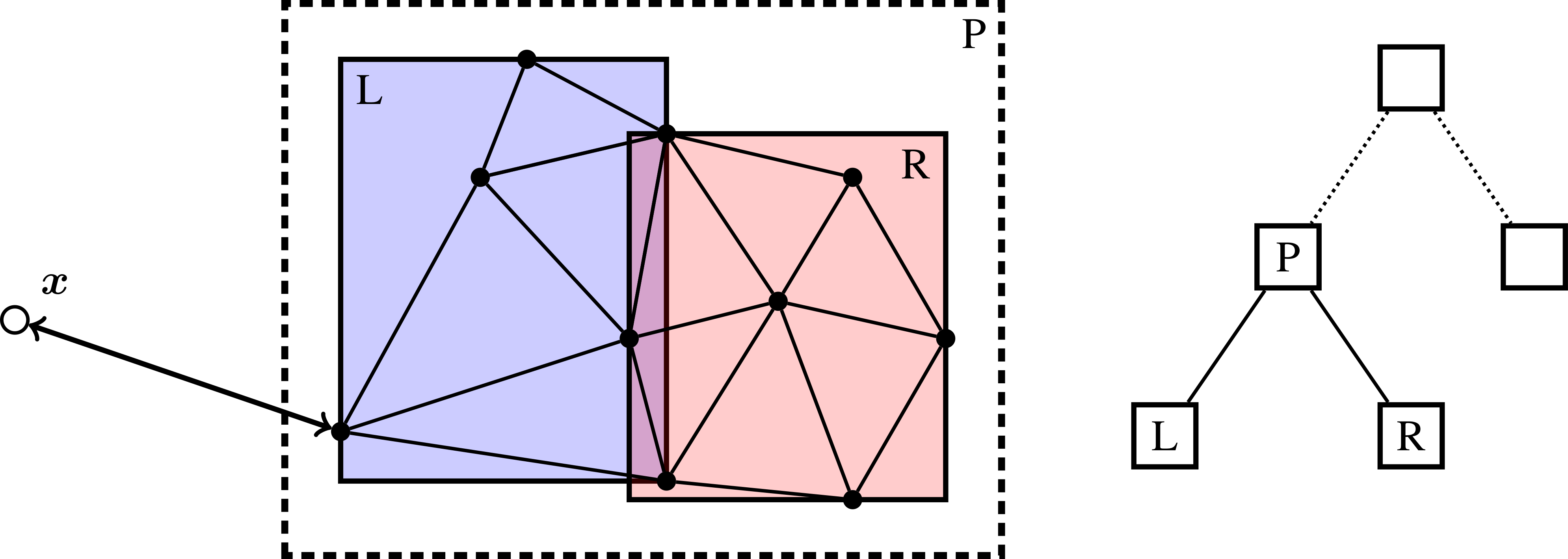
Fig. 4 Example of BVH partitioning for enclosing triangles. The regular node \(P\) contains two leaf nodes \(L\) and \(R\) which contain the primitives (triangles).
There is no fundamental limitation to what type of primitives/objects can be enclosed in BVHs, which makes BVHs useful beyond triangulated data sets. For example, analytic signed distance functions can also be embedded in BVHs, provided that we can construct bounding volumes that enclose them.
Important
EBGeometry is not limited to binary trees, but supports \(k\)-ary trees, where each regular node has \(k\) child nodes.
Construction
BVH construction is fairly flexible. For example, the child nodes \(L\) and \(R\) in Fig. 4 could be partitioned in any number of ways, with the only requirement being that each child node gets at least one triangle/primitive.
Although the rules for BVH construction are highly flexible, performant BVHs are completely reliant on having balanced trees with the following heuristic properties:
Tight bounding volumes that enclose the primitives as tightly as possible.
Minimal overlap between the bounding volumes.
Balanced, in the sense that the tree depth does not vary greatly through the tree, and there is approximately the same number of primitives in each leaf node.
Construction of a BVH is often done recursively, from top to bottom (so-called top-down construction). In this case, the BVH construction of a \(k\)-ary tree can be represented through a single function:
where \(\vec{O}\) is the input list of objects/primitives, which is partitioned into \(k\) new lists of primitives. Note that the lists \(\vec{O}_i\) do not contain duplicates; there is a unique set of primitives associated with each new leaf node. Top-down construction can thus be illustrated as a recursive procedure:
topDownConstruction(Objects):
   partitionedObjects = Partition(Objects)

   forall p in partitionedObjects:
      child = insertChildNode(newObjects)

      if(enoughPrimitives(child)):
         child.topDownConstruction(child.objects)
In practice, the above procedure is supplemented by more sophisticated criteria for terminating the recursion, as well as routines for creating the bounding volumes around the newly inserted nodes. EBGeometry implements top-down construction using a user-supplied partitioning rule (the \(\mathrm{Partition}\) above) and a termination criterion. Several ready-made partitioning strategies are provided, splitting on bounding-volume centroids (the default) or on primitive centroids; a more expensive strategy based on the Surface Area Heuristic typically yields the best query performance, at a higher construction cost.
Bottom-up construction is also possible, in which case one constructs the leaf nodes first, and then merges the nodes upward until one reaches a root node. In EBGeometry, bottom-up construction is done by means of space-filling curves – Morton codes, Hilbert curves, or nested indices. The Hilbert curve has better spatial locality than Morton (its consecutive codes are always spatially adjacent), so it tends to produce tighter leaf groupings.
Important
BVHs do not need to be stored with pointer referencing between nodes; it is quite possible to pack nodes tightly in memory on a linear array with direct indexing. This is useful when applying SIMD instructions for querying multiple bounding volumes simultaneously.
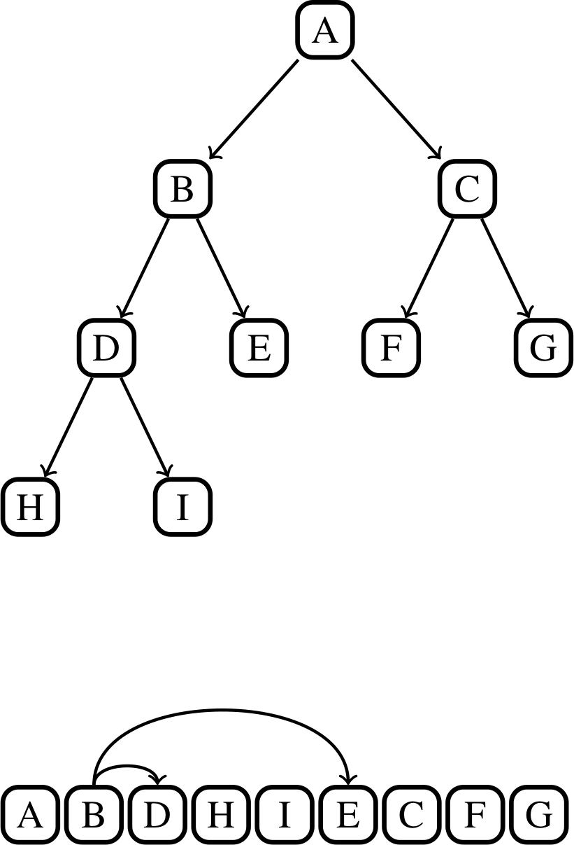
Fig. 5 A pointer-based tree (top) and an equivalent, flattened representation of the same tree (bottom). The tree is traversed top-to-bottom along its branches and laid out in that same order in a linear array; each interior node then stores index offsets to its children within the array, rather than pointers.
Refitting
Once a BVH has been built, its tree topology – which primitive lives in which leaf, and how the nodes nest – is independent of where the primitives actually sit in space. If a geometry moves slightly (a rigid displacement, or a small per-primitive jitter between frames) the topology is still perfectly usable; only the bounding volumes have gone stale. Refitting exploits this: it walks the tree from the leaves up, recomputing each leaf’s bounding volume from its (now moved) primitives and each interior node’s volume as the union of its children’s, without re-partitioning anything. This is far cheaper than a full rebuild and is the standard way to keep a BVH valid for a moving geometry.
The trade-off is quality rather than correctness: a refitted tree always encloses its primitives
(so traversal stays correct), but because the partitioning is frozen, a geometry that deforms enough
for primitives to drift into what used to be a neighbour’s region produces increasingly loose,
overlapping bounding volumes and slower queries. A periodic rebuild restores tight volumes once the
deformation has grown large. See BVH for the concrete refit() member functions
on both BVH representations.
Tree traversal
When computing the signed distance function to objects embedded in a BVH, one takes advantage of the hierarchical embedding of the primitives. Consider the case in Fig. 6, where the goal of the BVH traversal is to minimize the number of branches and nodes that are visited. For the traversal algorithm we consider the following steps:
When descending from node \(P\) we determine that we first investigate the left subtree (node \(A\)) since its bounding volume is closer than the bounding volumes for the other subtree. The other subtree is investigated after we have recursed to the bottom of the \(A\) subtree.
Since \(A\) is a leaf node, we compute the signed distance from \(\mathbf{x}\) to the primitives in \(A\). This requires us to iterate over all the triangles in \(A\) – it is often beneficial to use an SoA layout for the triangles so this calculation can be vectorized.
When investigating the other child node of \(P\), we find that the distance to the primitives in \(A\) is shorter than the distance from \(\mathbf{x}\) to the bounding volume that encloses nodes \(B\) and \(C\). This immediately permits us to prune the entire subtree containing \(B\) and \(C\), and there is never any need to compute the distance between \(\mathbf{x}\) and the triangles in this subtree.
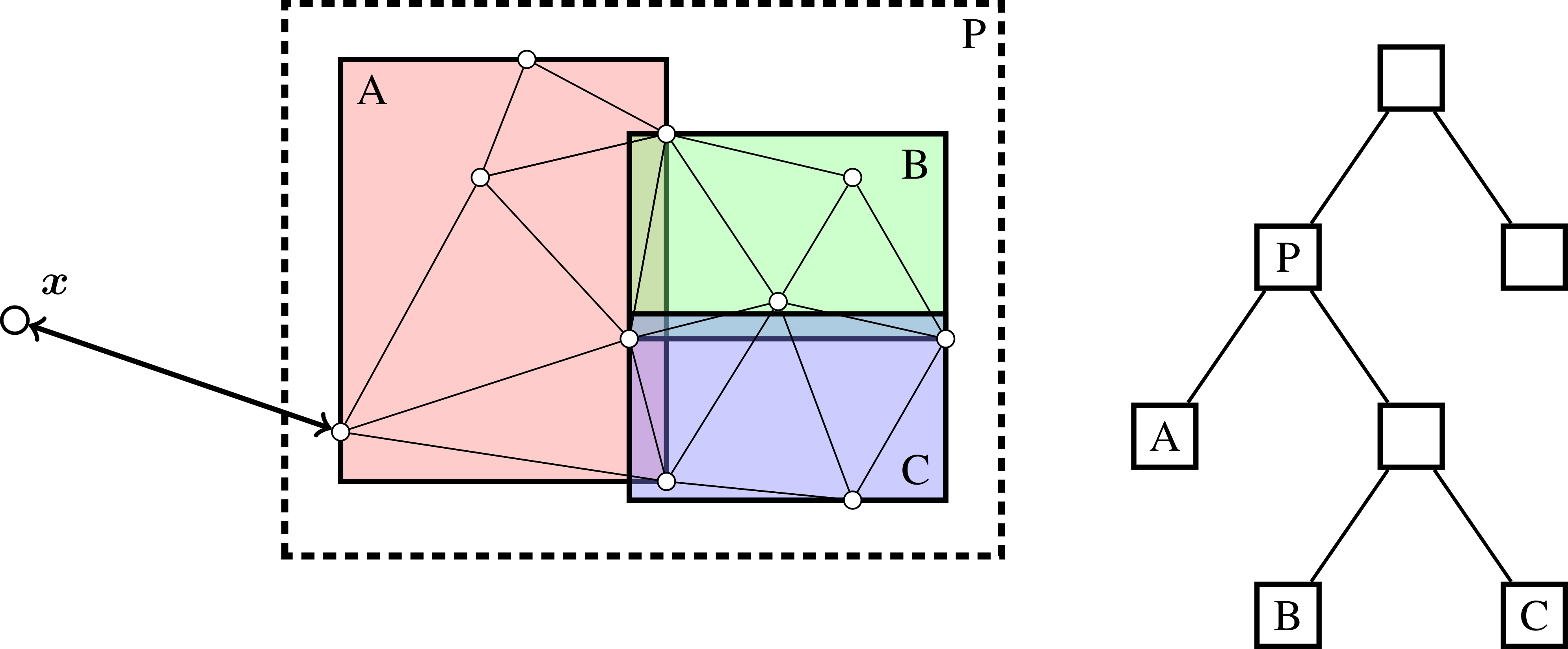
Fig. 6 Example of BVH tree pruning.
Other types of tree traversal, that do not compute a signed distance, are also possible. EBGeometry supports a fairly flexible approach to the tree traversal and update algorithms, so that the same hierarchical traversal-and-pruning idea can also be used for other operations – for instance, finding every facet within a specified distance of a point uses exactly the same principle.
Warning
BVH traversal has \(\log N\) complexity on average. However, in the worst case the traversal algorithm may have linear complexity if the primitives are all at approximately the same distance from the query point. For example, it is necessary to traverse almost the entire tree when one tries to compute the signed distance at the origin of a tessellated sphere since all triangles and their bounding volumes are approximately at the same distance from the center.