Half-edge meshes (DCEL)

Principle

EBGeometry uses a doubly-connected edge list (DCEL) structure – also known as a half-edge mesh – for storing surface meshes. The DCEL structures consist of the following objects:

• Planar polygons (facets).

• Half-edges.

• Vertices.

As shown in Fig. 1, half-edges circulate the inside of the facet, with knowledge of the next half-edge. A half-edge also stores a reference to its starting vertex, as well as a reference to its pair-edge. From the DCEL structure we can obtain all edges or vertices belonging to a single facet by iterating through the half-edges, and also jump to a neighboring facet by fetching the pair edge.

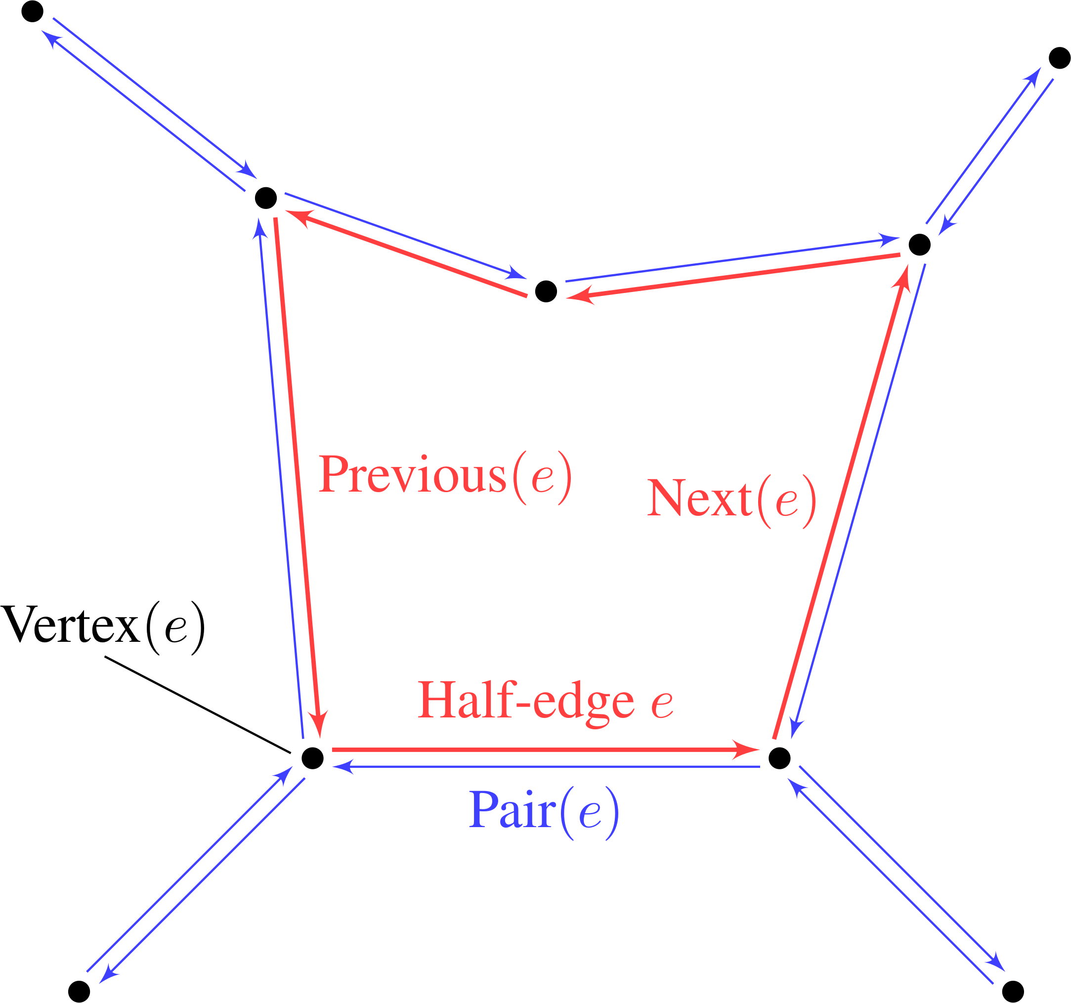
Fig. 1 DCEL mesh structure. Each half-edge stores references to next half-edge, the pair edge, and the starting vertex. Vertices store a coordinate as well as a reference to one of the outgoing half-edges.

While a DCEL mesh usually only requires storage of the edge structure, one can turn a DCEL mesh into a signed distance field by also storing normal vectors on each of the primitives, as indicated in the table below.

Concept	Stores
Vertex	Position, pseudonormal, one outgoing half-edge.
Half-edge	Owning face, next edge, pair edge, starting vertex, pseudonormal.
Facet	One boundary half-edge, face normal, a 2D embedding of the polygon, centroid.

Important

A signed distance field requires a watertight and orientable surface mesh. If the surface mesh consists of holes or flipped facets, neither the signed distance nor the implicit function exists. If the mesh contains such deficiencies, or is self-intersecting, only the unsigned distance is well-defined.

Signed distance

The signed distance to a surface mesh is equivalent to the signed distance to the closest polygon face in the mesh. When computing the signed distance from a point \(\mathbf{x}\) to a polygon face (e.g., a triangle), the closest feature on the polygon can be one of the vertices, edges, or the interior of the polygon face, see Fig. 2.

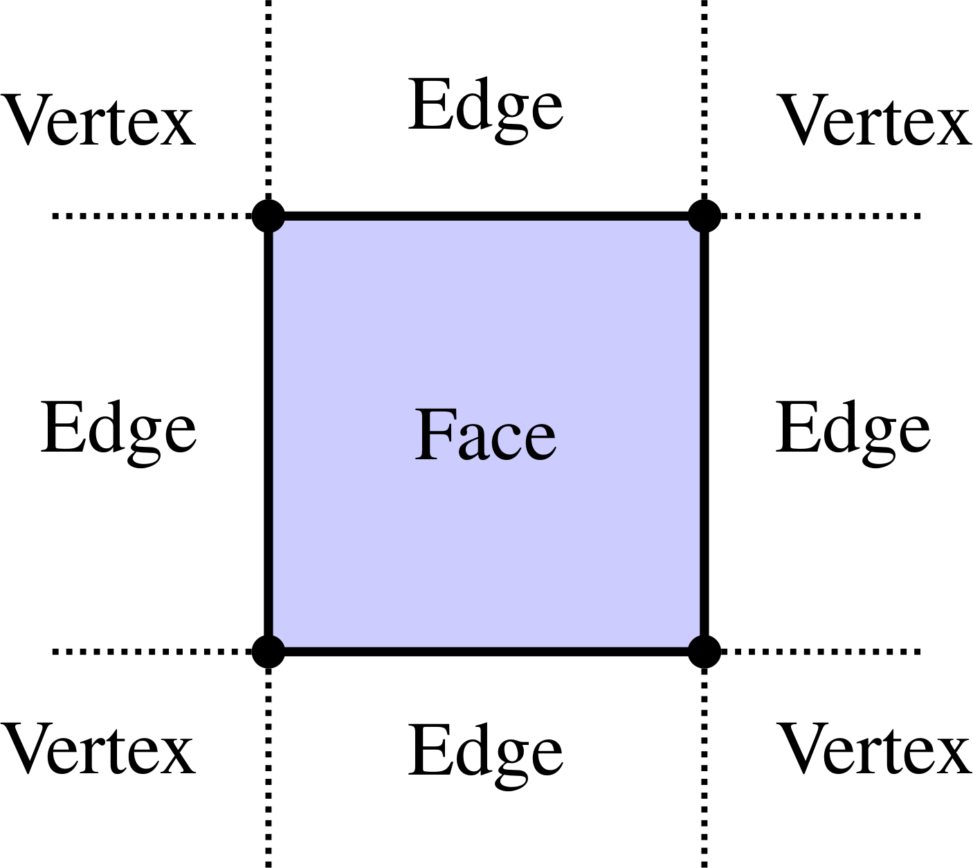
Fig. 2 Possible closest-feature cases after projecting a point \(\mathbf{x}\) to the plane of a polygon face.

Three cases can be distinguished, and each has a direct counterpart in the DCEL structure: a vertex, a half-edge, and a facet can each be asked for both the signed distance \(d = S(\mathbf{x})\) and the squared unsigned distance \(d^2\) to a query point, where the latter avoids a square root when only the closest feature (not the exact distance to it) needs to be determined – this is the quantity used for comparisons when descending through a bounding volume hierarchy, see Bounding volume hierarchies.

1. Facet/Polygon face.

   When computing the distance from a point \(\mathbf{x}\) to the polygon face we first determine if the projection of \(\mathbf{x}\) to the face plane lies inside or outside the face. This is more involved than one might think, and it is done by first computing the two-dimensional projection of the polygon face, ignoring one of the coordinates. Next, we determine, using 2D algorithms, if the projected point lies inside the embedded 2D representation of the polygon face. Various algorithms for this are available, such as computing the winding number, the crossing number, or the subtended angle between the projected point and the 2D polygon. The 2D embedding itself is computed once, at mesh-construction time, and reused for every subsequent query.

   Tip

   EBGeometry uses the crossing number algorithm by default.

   If the point projects to the inside of the face, the signed distance is just \(\mathbf{n}_f\cdot\left(\mathbf{x} - \mathbf{x}_f\right)\) where \(\mathbf{n}_f\) is the face normal and \(\mathbf{x}_f\) is a point on the face plane (e.g., a vertex). If the point projects to outside the polygon face, the closest feature is either an edge or a vertex.

2. Edge.

   When computing the signed distance to an edge, the edge is parametrized as \(\mathbf{e}(t) = \mathbf{x}_0 + \left(\mathbf{x}_1 - \mathbf{x}_0\right)t\), where \(\mathbf{x}_0\) and \(\mathbf{x}_1\) are the starting and ending vertex coordinates. The point \(\mathbf{x}\) is projected to this line, and if the projection yields \(t^\prime \in [0,1]\) then the edge is the closest point. In that case the signed distance is the projected distance and the sign is given by the sign of \(\mathbf{n}_e\cdot\left(\mathbf{x} - \mathbf{x}_0\right)\) where \(\mathbf{n}_e\) is the pseudonormal vector of the edge. Otherwise, the closest point is one of the vertices.

3. Vertex.

   If the closest point is a vertex then the signed distance is simply \(\mathbf{n}_v\cdot\left(\mathbf{x}-\mathbf{x}_v\right)\) where \(\mathbf{n}_v\) is the vertex pseudonormal and \(\mathbf{x}_v\) is the vertex position.

The mesh-level signed distance is then the minimum, in the unsigned-squared sense, over every facet’s contribution, taking a final square root only once the closest facet has been identified. Scanning every facet this way works but has \(\mathcal{O}(N)\) complexity for \(N\) facets; Bounding volume hierarchies describes how the query cost can be reduced dramatically by embedding the facets in a bounding volume hierarchy.

Normal vectors

The normal vectors for edges \(\mathbf{n}_e\) and vertices \(\mathbf{n}_v\) are, unlike the facet normal, not uniquely defined. For both edges and vertices we use the pseudonormals from [1]:

\[\mathbf{n}_{e} = \frac{1}{2}\left(\mathbf{n}_{f} + \mathbf{n}_{f^\prime}\right).\]

where \(f\) and \(f^\prime\) are the two faces connecting the edge. The vertex pseudonormal is given by

\[\mathbf{n}_{v} = \frac{\sum_i\alpha_i\mathbf{n}_{f_i}}{\left|\sum_i\alpha_i\right|},\]

where the sum runs over all faces which share \(v\) as a vertex, and where \(\alpha_i\) is the subtended angle of the face \(f_i\), see Fig. 3.

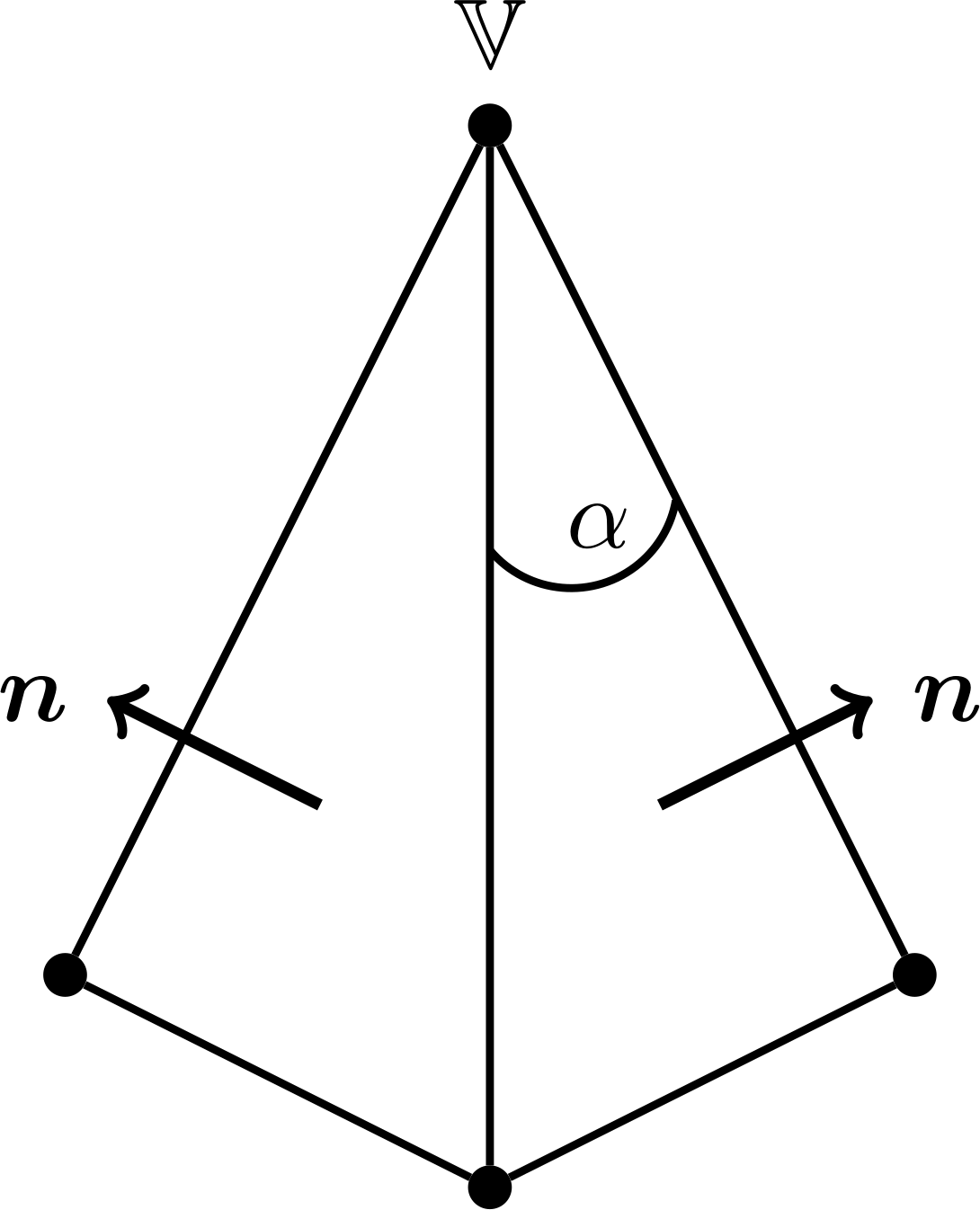
Fig. 3 Edge and vertex pseudonormals.

Both pseudonormals are computed once, at mesh construction time, and then simply stored and reused by every subsequent distance query.